The Environmental Analyst

A Short History of Wolves in America

Posted on October 17, 2013 | Leave a comment

The question before us is: should wolves in the United States be taken off the Endangered Species List? To analyze this question, we need to review the history of wolves in America.

The number of wolves living in North America before the arrival of Europeans is estimated at 400,000 animals¹. As white Americans and their livestock migrated westward in the 19th century, they came in conflict with wolves. Various states offered bounties for dead wolves, and the U.S. Government waged its own campaign against wolves beginning in 1914². Wolves were gone from western states by the 1930’s and from Wisconsin and Michigan by the mid-1960’s³. By that time, the only wolves remaining in the lower 48 states resided in Minnesota³.

With the rise of the conservation and environmental movements in the U.S. in the 1960’s, attitudes towards the wolf began to change. After passage of the Endangered Species Preservation Act (1966), eastern wolves (Canis lupus lycaon) and red wolves (Canis rufus) were listed as endangered in 1967⁴. With the Endangered Species Act passing in 1973, four subspecies of wolves were granted protection in 1974)³. The entire species of gray wolf was granted protection in 1978, designated as endangered, except in Minnesota where the species was designated as threatened³.

Once they fell under Federal protection, wolves could no longer be killed at whim, and they began to infiltrate into northern United States from Canada⁵. As far as I can tell, the vast majority of wolves are concentrated in northern states⁶. While sightings of lone wolves have been reported in many states, a wolf population can not be considered established in a particular area until the presence of at least one pack has been documented. To my knowledge, as of October 2013 there are very few documented packs living in the wild south of 42° latitude, except for red wolves and Mexican gray wolves⁷.

The vast majority of wolves in the U.S. are concentrated in five regions. These areas are ⁸ (followed by best estimates of population):

Alaska 7,700 to 11,200
Western Great Lakes 3,686
Northern Rocky Mountains 1,674
Southwest (Mexican wolves in the Blue Range Recovery Area) 75
North Carolina (Red wolves in the Alligator River National Wildlife Refuge) 100

In particular, the wolves in the Western Great Lakes region and the wolves in the Northern Rocky Mountains region are designated distinct population segments (DPS) by the Fish and Wildlife Service⁹.

The following map from Defenders of Wildlife shows the range of wolves in the North American continent, past and present¹⁰. The map is shaded as follows:

Dark greening shading is where gray wolves live currently.
Light green shading is where gray wolves have lived in the past.
Red shading is where red wolves live currently (North Carolina).
Red-spotted shading is where red wolves have lived in the past.
Red-striped areas are currently suitable wolf habitat where wolves do not live now but could migrate there.

Here is the map:

Wolves have always lived in Alaska and Canada and were never endangered¹¹. Once protection was afforded to wolves in the lower 48 states (wolves never lived in Hawaii¹²), they started to cross the northern U.S. border from Canada⁵. Wolves were never completely eradicated from northern Minnesota¹³, and as their numbers recovered they gradually spread to Wisconsin and the Upper Peninsula of Michigan¹⁴ to found the Western Great Lakes DPS. Below is a map showing their current range in the Western Great Lakes region¹⁵:

Wolves moving into Montana’s National Glacier Park formed the Northern Rocky Mountains DPS. They were joined by wolves that were captured in Canada and released in Yellowstone National Park (31 wolves) and central Idaho (35 wolves) in 1995 and 1996¹⁶. Here is a map showing wolf packs in the northern Rocky Mountain region¹⁷:

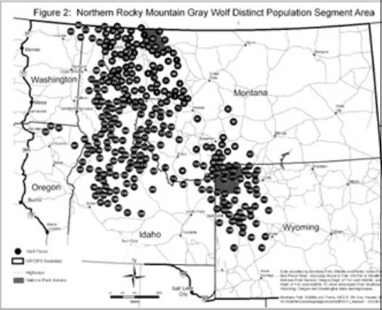
Notice that this region has actually two centers of population: the area straddling the Idaho-Montana border, and a second area centered on Yellowstone Park. There are packs between these two areas, but they are much less concentrated.

I thought it might be instructive if I also showed maps of Wyoming, Montana, and Idaho. First, a map of Wyoming. Wyoming has four important areas¹⁸:

The extreme northwest corner of the state is Yellowstone National Park, where hunting is not allowed.
The area surrounding the park (outlined in the map in green) is the Trophy Game Management Area, where wolves can be hunted by licensed hunters during a designated season (October 1 through December 31) up to an area-wide quota.
A small area south of the park called the Seasonal Wolf Trophy Game Management Area (outlined in the map in red), where hunting in the area is divided into three periods:

January 1 through last day in February. No hunting allowed.
March 1 through October 14. Wolves can be killed by anybody at anytime without limit.
October 15 through December 31. Hunting by licensed hunters only up to an area-wide quota.

The rest of the state, where wolves can be killed by anybody at anytime without limit.

Here is the map. The area bordered in green is the trophy area. The area bordered in red is the seasonal trophy area¹⁸:

Here is a map of wolves in Montana¹⁹, most of which are in the western third of the state:

Here is a map of wolves in Idaho²⁰, whose activity takes up most of the northern two-thirds of the state:

The Mexican gray wolf (Canis lupus baileyi) was nearly exterminated from its range in the southwestern U.S. by the 1970’s. In 1998, wolves were released into the Blue Range Wolf Recovery Area (BRWRA) as a nonessential experimental population²¹, that is, a population of animals reintroduced into the area whose survival is not essential to the survival of the species as a whole. The nonessential experimental designation relaxes some of the burdens that the Endangered Species Act places on nearby landowners in the hope of reducing opposition to the reintroduction²². The following map shows the Blue Range Wolf Recovery Area surrounded by the much larger Mexican Wolf Experimental Population Area²³:

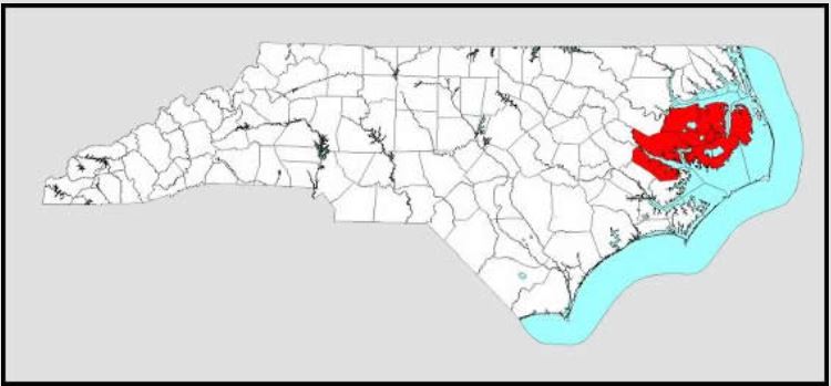
Red wolves (Canis rufus) are a separate species with an historical range that included all of the southeast U.S., going as far north as Pennsylvania and the Ohio river valley and as far west as Texas²⁴. Red wolves were extinct from the wild by 1970, except for a small population that was discovered near the Gulf coast straddling the Texas-Louisiana border. The U.S. Fish and Wildlife Service captured as many animals from this population as it could, and selected 14 individuals for a captive breeding program²⁵. In 1987, descendents of these animals were released into the Alligator River National Wildlife Refuge (ARNWR)in eastern North Carolina near the Outer Banks²⁶. Most red wolves in the wild currently reside in or near the ARNWR, as shown in this map from the Fish and Wildlife Service²⁷:

In the past few years, the U.S. Fish and Wildlife Service (FWS) has moved to delist wolves from endangered status²⁸. The Northern Rocky Mountain DPS (except in Wyoming) was delisted in May 2011²⁹, the Western Great Lakes DPS was delisted in December 2011³⁰, and wolves in Wyoming were delisted in August 2012²⁹. Mexican wolves in the Blue Range Recovery Area and red wolves remain under protection with no plans to change their status. All other wolves in the contiguous U.S. remain under protection, but in June 2013, the FWS announced its intention to remove this protection³¹, and it is this announcement which is the source of the controversy we now considering.

In place of Federal protection, the FWS has signed Memoranda of Agreement with Montana, Idaho, and Wyoming³². All these states³³ and Oregon, Washington, Colorado, Utah³⁴, Minnesota, Michigan, and Wisconsin³⁵ have state wolf management plans to conserve their wolf populations while minimizing conflicts with humans.

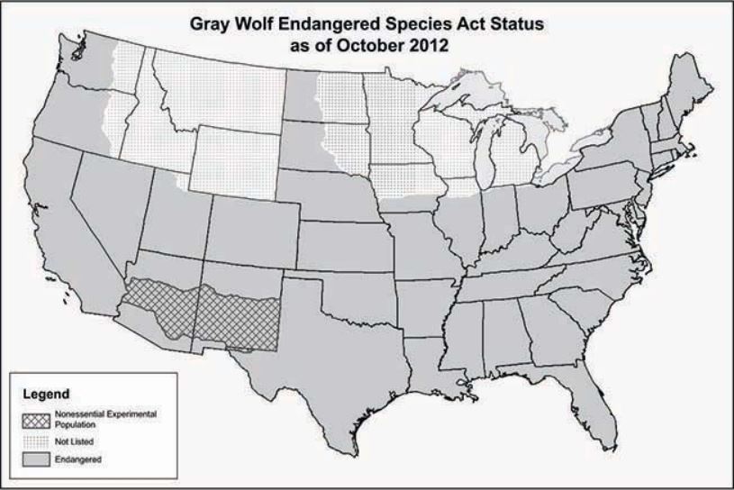
The following map from the U.S. Fish and Wildlife Service shows current endangered species status across the states³⁶:

In my next post, I will discuss the delisting of the wolf from Endangered Species List.

Footnotes

Defenders of Wildlife, Places for Wolves: A Blueprint for Restoration and Recovery in the Lower 48 States, 2006, p. 6. To view the document, click here.
International Wolf Center website, Gray Wolf Time Line for the Contiguous United States. To view, click here.
Minnesota Department of Natural Resources website, Canis lupus Gray Wolf. To view, click here.
U.S. Fish and Wildlife Service website, First Species Listed as Endangered. To view, click here. Note that the scientific name for the red wolf is given as Canis niger rather than Canis rufus.
Mission: Wolf, A History of Wild Wolves in the United States. To view, click here. Montana Fish, Wildlife, & Parks website, Gray Wolf History. To view, click here.
See map below.
I came to this conclusion after examining several states, such as California, that have suitable wolf habitat but no record of resident wolf packs. I am open to correction on this point.
U.S. Fish and Wildlife Service website, Gray Wolf (Canis lupis) Current Population in the United States. To view, click here.
U.S. Fish and Wildlife Service website, Species Profile: Gray Wolf (Canis lupis). To view, click here.
Defenders of Wildlife, Places for Wolves: A Blueprint for Restoration and Recovery in the Lower 48 States, 2006, p. 15. To view the document,click here.
U.S. Fish and Wildlife Service website, Wolf Recovery Under the Endangered Species Act, p. 2. To view, click here.
I came to this conclusion through deduction, although I did find a website page I believe once belonged to the Hawaii Department of Land and Natural Resources but is now obsolete, entitled Are there bears or wolves in Hawaii? To view, click here.
U.S. Fish and Wildlife Service website, Gray Wolf Recovery in Minnesota, Wisconsin, and Michigan. To view, click here. Minnesota Department of Natural Resources website, Canis lupus Gray Wolf. To view, click here.
U.S. Fish and Wildlife Service website, Gray Wolf Recovery in Minnesota, Wisconsin, and Michigan. To view, click here.
U.S. Fish and Wildlife Service website, Gray Wolf — Western Great Lakes Distinct Population Segment. To view, click here.
Montana Fish, Wildlife, and Parks website, Gray Wolf History. To view, click here. There is an excellent video on scientific research of wolves in Yellowstone National Park, entitled NATURE | The Wolf That Changed America | Wolf Expert | PBS which you can view by clicking here.
U.S. Fish and Wildlife website, Gray Wolves in the Northern Rocky Mountains: News, Information and Recovery Status Reports. To view, click here.
Wyoming Game & Fish Department website, Wolves in Wyoming. To view, click here.
State of Montana website, Montana Field Guide: Gray Wolf — Canis Lupus. To view, click here.
Idaho Fish and Game Department, 2012 Idaho Wolf Monitoring Progress Report, p. 12. To view, click here.
U.S. Fish and Wildlife website, Mexican Gray Wolf Recovery Program History. To view, click here.
U.S. Fish and Wildlife website, Topeka Shiner Reintroduction in Missouri; Designation of Non-Essential, Experimental Population: Questions and Answers. To view, click here. U.S. Fish and Wildlife Service, Endangered Species Act: Experimental Populations. To view, click here.
U.S. Fish and Wildlife Service website, Mexican Wolf Experimental Population Area (map showing 10(j) boundary). To view, click here.
U.S. Fish and Wildlife Service, Endangered Red Wolves, p. 3. To view, click here. It is interesting that FWS shows a map of the red wolf’s historical range that plots it as far north as Massachusetts, southern New York, most of Pennsylvania, Ohio, and Indiana, and half of Illinois and Missouri. Click here to view. Indeed, a serious claim that red wolves inhabited the Adirondacks area in Northern New York State was made in an Adirondack Citizen Advisory Committee report on the possible reintroduction of wolves into Adirondack Park, as reported on the Defenders of Wildlife website, Wolves in the Adirondacks?, which you can view by clicking here.
U.S. Fish and Wildlife Service, Endangered Red Wolves, p. 1. To view, click here.
U.S. Fish and Wildlife Service, Endangered Red Wolves, pp. 2, 6–7 To view, click here. U.S. Fish and Wildlife Service website, Recovery Timeline. To view, click here.
U.S. Fish and Wildlife Service website, Red Wolf Recovery Efforts. To view, click here. There is a fascinating discussion in Wikipedia on the controversy whether the red wolf is a true species or is merely a hybrid of gray wolves and coyotes, which you can view by clicking here and scrolling down to the section “Taxonomy.”
U.S. Fish and Wildlife Service website, Species Profile: Gray Wolf (Canis lupis), section “Current Listing Status Summary” and further to the end of the page. To view, click here.
U.S. Fish and Wildlife Service website, Gray Wolves in the Northern Rocky Mountains: News, Information, and Recovery Status Reports, section “Recent Actions:”. To view, click here.
U.S. Fish and Wildlife Service website,Gray Wolves in the Western Great Lakes States, section “Chronology of Federal Actions Affecting Gray Wolf ESA Status in the Western Great Lakes States.” To view, click here.
U.S. Fish and Wildlife Service website,Gray Wolves in the Western Great Lakes States, section “June 7, 2013 Announcement.” To view,click here. There is no indication anywhere on the U.S. Fish and Wildlife Service website that the red wolf is proposed for delisting.
U.S. Fish and Wildlife Service website, Gray Wolves in the Northern Rocky Mountains: News, Information, and Recovery Status Reports, section “Wolf Management Memorandums of Agreement”. To view, click here.
U.S. Fish and Wildlife Service website, Gray Wolves in the Northern Rocky Mountains: News, Information, and Recovery Status Reports, section “State Wolf Management in Idaho, Montana, and Wyoming”. To view, click here.
U.S. Fish and Wildlife Service website, Gray Wolves in the Northern Rocky Mountains: News, Information, and Recovery Status Reports, section “Other State and Tribal Wolf Management”. To view, click here.
U.S. Fish and Wildlife Service website,Minnesota, Wisconsin, and Michigan State Management Plans. To view, click here.
U.S. Fish and Wildlife Service website, Gray Wolf – Western Great Lakes Region: Status under the Endangered Species Act. To view, click here.

Leave a comment

Posted in Wildlife Conservation, Wolves in America

Tagged Alaska, delisting, Endangered Species Act, gray wolves, Idaho, Mexican gray wolves, Michigan, Minnesota, Montana, North Carolina, Northern Rocky Mountains, red wolves, Southwest, U.S. Fish and Wildlife Service, Western Great Lakes, Wisconsin, wolf population, wolves, Wyoming, Yellowstone National Park

Why Wolves Are Important

Posted on August 22, 2013 | Leave a comment

When discussing the conservation of wolves, it is important to understand why we should bother to save wolves from extinction. They attack and eat livestock and pets, causing economic losses to farmers and ranchers and anguish to pet owners, and they compete with human hunters for game such as elk. Are they merely a pest species?

To answer this question, we need to know something about the scientific discipline of community ecology. In colloquial usage, ecology is another word for environmentalism, but as a scientific discipline, ecology is the broadest concern of biology, the science of life. Whereas other branches of biology are concerned with cells, organs, or individual animals and plants, community ecology studies how different species of plants, animals, and microorganisms interact with each other within a biological community. A community might be a forest, a stretch of desert, a national park, a portion of the seashore, someone’s backyard, and so on.

Most healthy, self-sustaining biological communities have four types of members:

Producers. These are either plants or green algae that convert non-living matter into organic substances that they incorporate into their bodies through the process of photosynthesis. They feed everyone else in the community, directly or indirectly.
Primary consumers. These organisms, mostly animals, eat the producers. Herbivores, such as cows, sheep, and elk, also plant-eating insects.
Predators. These organisms eat other consumers. Carnivores, such as mountain lions, wolves, snakes, and ladybug beetles.
Decomposers. Mostly microorganisms and fungi as well as insects that eat dung. They break down the tissues of dead plants and animals and animal excrement and make the chemicals found there available as food for the producers. Nature’s great recyclers.

All four classes of organisms are important to a healthy ecosystem. If one class is diminished, an imbalance occurs which disrupts the nutrient cycle, makes it harder for other species to thrive, and reduces biodiversity. For example, without decomposers like bacteria, dead plant and animal matter can’t be recycled for plants to use, and the nutrient cycle is disrupted. Without plants to make food, primary consumers cannot survive, and soon, neither can the predators that feed on them. Without predators, consumers become too numerous and become destructive of the plant species off which they feed.

National Public Radio’s Morning Edition Show recently broadcast a story on this topic entitled When Big Carnivores Go Down, Even Vegetarians Take The Hit. The broadcast is a little more than three minutes, and you can read it (and listen to it) by clicking here.

A good example of this discussion is the Yellowstone Park community. Wolves were exterminated there as they were in most of America in the 1920’s, but were reintroduced in 1995. First, here is a link to a video on the topic entitled Predators by Bill Ripple, which you can view by clicking here.

Here is an excellent essay on wolves in Yellowstone that appears on the website of the Wyoming chapter of the Sierra Club, which I am reprinting here, in compliance with the Sierra Club’s Terms and Conditions of Use. It was written by members of the Western Wolf Coalition. It explains what the wolf has done for the Yellowstone Park ecological community:

Ecological Benefit of Wolves

Wolves play a vital role in maintaining the health and sustainability of the landscape in the greater Yellowstone region and our western lands. They are a keystone species, one that has a disproportionate impact on its environment relative to its abundance. Since their return in 1995, wolves have benefitted this ecosystem by regulating prey numbers and movements—allowing streambank habitats to recover, reducing densities of coyotes, and providing food for scavengers.

The most recognized and well-documented ecological benefit of wolves is that they have resumed the important role of maintaining healthy wildlife herds in the northern Rockies by selecting young, old, physically impaired, or diseased animals⁵. By reducing prey numbers, dispersing these animals on the landscape, and removing sick animals, wolves also may reduce the transmission and prevalence of wildlife diseases such as chronic wasting disease and brucellosis⁷.

In addition to improving the overall fitness of wildlife herds, wolves have also altered the behavior of their prey, leading to a cascade of beneficial effects on the landscape. In the absence of wolves, elk tended to browse heavily in the open flats along rivers and wetlands, since they did not need to evade predators by seeking thicker cover. Without fear of wolves, elk over-browsed the vegetation inhibiting the growth of new trees. Since the reintroduction of wolves in Yellowstone, elk spend more time in the safety of thick cover or on the move⁶. As a result, riparian areas and aspen groves that had been suppressed by decades of over-browsing are regenerating, improving habitat for species like beavers and songbirds³. Beavers, which create wetland habitats with their dams, have improved water quality in streams by trapping sediment, replenishing groundwater, and cooling water.

Species that rely on healthy riparian habitats and benefit from the presence of wolves in Yellowstone National Park include:

Yellowstone cutthroat trout and other native fish
Moose
Waterfowl (ducks, geese, trumpeter swans)
Songbirds (such as warblers, wrens, and thrushes)
Small mammals (such as beavers, muskrats,
and other rodents)
Insects, amphibians, and countless other species^3,6

Wolves and Coyotes

In the absence of wolves, coyotes became a top predator in the ecosystem, but they are not large enough to regulate elk, deer, and moose populations². The return of the wolf restored a natural complement of predators to northwest Wyoming and returned the coyote to its role as a mid-level predator. Wolves will kill coyotes and outcompete them at kill sites. Coyotes also prey heavily on pronghorn fawns. Since wolves returned to the landscape, pronghorn populations have increased in northern Yellowstone as a result of declining coyote populations and densities ¹.

Wolves and Scavengers

Scavengers, such as ravens, eagles, and bears, also benefit heavily from the return of wolves. Wolf kills provide scavengers with an important source of protein, particularly in winter. Twelve species of scavengers are known to visit wolf kills in Yellowstone National Park ¹⁰. Ravens are especially attuned to wolves and may fly over wolf packs as they pursue prey, allowing them quick access to wolf kills. In turn, wolves may benefit from ravens by following them to carcasses that can feed both species⁸.

Prior to the reintroduction of wolves, scavengers were more dependent on animals that died due to harsh winters. Since snow is thawing earlier as a result of a warming climate, there are fewer winter kills available for scavengers. Wolf kills may help buffer the impacts of climate change for scavengers by providing them with a food source in the winter⁹.

Conclusions

The return of the wolf to Wyoming has had significant ecological benefits in a relatively short period of time. Ecological concerns contributed to the decision to return wolves and should play a role in how states manage this keystone species. Although it is easy to focus on the perceived negative impacts of wolves, it is important to recognize the actual benefits they provide to our ecosystem. By regulating wildlife herds and reducing the prevalence of diseases, revitalizing riparian areas, reducing coyote densities, providing food for scavengers, and indirectly improving conditions for a host of other species, wolves play an essential role in maintaining the ecological health and integrity of the landscape.

Footnotes to this article

Berger, K.M., E.M. Gese and J. Berger. 2008. Indirect effects and traditional trophic cascades: A test involving wolves, coyotes, and pronghorns. Ecology 89:818-828.
Berger, K.M. and E.M. Gese. 2007 Does interference competition with wolves limit the distribution and abundance of coyotes? Journal of Animal Ecology 76:1075-1085.
Cooke, H.A. and S. Zack. 2008. Influence of beaver dam density on riparian areas and riparian birds in shrub steppe of Wyoming. Western North American Naturalist 68: 350-364.
Halofsky, J.S., W.J. Ripple and R.L. Bestcha. 2008. Recoupling fire and aspen recruitment after wolf reintroduction in Yellowstone National Park, USA. Forest ecology and management 256(5):1004-1008.
Mech L.D., D.W. Smith, K. M. Murphy, and D. R. MacNulty. 2001. Winter severity and wolf predation on a formerly wolf-free elk herd. Journal of Wildlife Management 65:998-10
Ripple, W.J. and R.L. Bestcha. 2006. Linking wolves to willows via risk-sensitive foraging by ungulates in the northern Yellowstone ecosystem. Forest ecology and management 230(1-3):96-106.
Smith, B.L. 2005. Disease and Winter Feeding of Elk and Bison: A Review and Recommendations Pertinent to the Jackson Bison and Elk Management Plan and Environmental Impact Statement.
Stahler, D.R., B. Heinrich and D.W. Smith. 2002. Common ravens, Corvus corax, preferentially associate with grey wolves, Canis lupus, as a foraging strategy in winter. Animal Behaviour 64(2):283.
Wilmers, C.C. and W.M. Getz . 2005. Gray wolves as climate change buffers in Yellowstone. PLoS Biology 3:571.
Wilmers, C.C., D.R. Stahler, R.L. Crabtree, D.W. Smith and W.M. Getz. 2003. Resource dispersion and consumer dominance: scavenging at wolf- and hunter-killed carcasses in Greater Yellowstone, USA. Ecology Letters 6:996–10

I also came across another excellent article on wolf ecology, this one entitled Wolves As Engineers of Biodiversity, published by the California Wolf Center, which I won’t reprint but you can view by clicking here.

Leave a comment

Posted in Wildlife Conservation, Wolves in America

Tagged community ecology, conservation, Defenders of Wildlife, ecology, Sierra Club, wildlife conservation, wolves

Topic: Should the Wolf Be Removed From the Endangered Species List?

Posted on August 22, 2013 | 2 comments

This post begins a new topic: Should the wolf be removed from the list of animals protected by the Endangered Species Act (ESA)? The topic consists of five posts. If you came here via a link, you can navigate between posts by clicking on the arrows that appear above the post heading. The right arrow (→) always points to the next post; the left arrow (←) always points to the previous post. In this particular post, the right arrow is labeled Why Wolves are Important and points to the next post. The left arrow is labeled Gun Homicides vs. Gun Ownership and points to a previous topic.

The last three posts have footnotes which list my sources but also have additional notes and links, so you might want to take a look at them.

If you have a comment, please feel free to type it on the bottom of the post, or send an email to mhkblogs@gmail.com . All constructive criticism is most welcome!

Recently, I received an email from the Natural Resources Defense Council (NRDC):

Dear Michael,

The future of America’s wolves is in jeopardy

The Obama Administration’s new proposal would scrap vital protections for gray wolves across most of the Lower 48 states. Help us send one million messages of opposition to this disastrous plan and give wolves a fighting chance at recovery!

The clock is ticking down for our nation’s wolves.

The Obama Administration has given the public just 90 days to comment on its disastrous plan to strip wolves of their vital Endangered Species Act protections across most of the Lower 48 states.

NRDC and other conservation groups have set an ambitious goal of generating one million messages of protest to stop this far-reaching assault on wolves.

Please do your part by telling the U.S. Fish and Wildlife Service to reverse its reckless plan and give wolves a fighting chance at recovery!

The return of gray wolves to areas like the Northern Rockies and the western Great Lakes has been one of the greatest conservation success stories of our time.

But wolves are only starting to return to large portions of their former range, like the Pacific Northwest. Lone wolves have crossed into California, Utah, Colorado and states in the Northeast.

Removing federal protections now would shut the door on wolf recovery long before the job is done.

This reckless plan, more the result of political pressure than sound science or policy, would throw national wolf recovery into reverse.

In fact, a group of the nation’s top wildlife scientists has sent a letter to the administration, objecting to its proposal.

Wolves will not recover unless they remain protected. That’s why it’s so critical that we keep the pressure on that agency to withdraw this horrendous plan.

Please send your message to the Fish and Wildlife Service right now. Call on them to keep wolves protected under the Endangered Species Act.

We’re at a crucial turning point in this fight — one that will determine whether wolves are allowed to survive and thrive in America. Thank you for making your voice heard in their defense.

Sincerely,

Frances Beinecke
President
Natural Resources Defense Council

I am not criticizing this request. It’s perfectly reasonable, and it asks citizens to speak up on behalf of a cause that they believe in. That is what democracy is all about. Nevertheless, the ad is wanting from a scientific perspective. It makes an assertion which it does not back up with evidence, although the evidence may indeed exist. That assertion is that while the wolf population in the lower 48 states has been allowed to recover, removing Endangered Species Act protections will reverse that recovery. As the email above puts it, “This reckless plan … would throw national wolf recovery into reverse. … Wolves will not recover unless they remain protected. … We’re at a crucial turning point in this fight — one that will determine whether wolves are allowed to survive and thrive in America.”

What is not clear from the email is what the Natural Resources Defense Council is predicting will happen if Endangered Species Act protection are lifted. Is it that wolf recovery will be arrested and wolf populations will be confined to where they exist now, or are they saying that the recovery is liable to being reversed, and that present wolf populations will shrink or disappear altogether? Let’s take a look at the position of wolves in America and estimate what might happen if Endangered Species Act protections are removed. But before we begin, let’s discuss why it is important to have wolves in our ecosystem in the first place, which in turn answers the question: why should we care? That will be the topic of my next post.

2 Comments

Posted in Wildlife Conservation, Wolves in America

Tagged conservation, Endangered Species Act, National Resources Defense Council, wildlife conservation, wolves

Topic: Gun Homicides vs. Gun Ownership

Posted on August 8, 2013 | 2 comments

This is a one-post topic examining the relationship between gun ownership and crimes committed with guns in America. Strictly speaking, this is not a concern of environmental science. But it is an issue that can be studied with the same sort of methods and analysis used by environmental science to tackle environmental problems, and therefore an appropriate topic for this blog.

Consider the following question: Is there a correlation between high rates of gun ownership and murders committed with firearms in the 50 states? To help answer it, I found three sets of data:

FBI 2010 crime statistics from their Unified Crime Reports (UCR).
U.S. Census Bureau 2010 statistics on population.
Washington Post, quoting a Center for Disease Control (CDC) 2001 survey on gun ownership.

The last source is problematic as it was done in 2001 rather than 2010. I’m assuming that gun ownership percentages did not change significantly between 2001 and 2010, but I could be wrong¹. It is also not an exact count but an estimation using samples. There is no official record of who is a gun owner in America. If you recall, the gun lobby is vehemently opposed to a national gun registry, and so we can only estimate the number of gun owners using surveys. This particular survey was conducted in all 50 states by the Centers for Disease Control’s Behavior Risk Factor Surveillance System. Respondents were chosen at random and were asked the following question: Are any firearms now kept in or around your home? Include those kept in a garage, outdoor storage area, car, truck, or other motor vehicle.

Therefore, when the survey states that 41.7% of respondents in Missouri claimed to have a firearm in the household in 2001, it doesn’t necessarily mean that 41.7% of all households in Missouri have firearms. There is a confidence interval or margin of error surrounding the sample statistic within which the true percentage is likely to fall. For example, suppose the 95% confidence level is plus or minus 3%. Then if 41.7% of the Missouri sample answered yes to the question, I can claim with 95% confidence (that is, I expect to be right 19 times out of 20) that the true percentage of Missouri households possessing firearms is somewhere between 38.7% and 44.7%. I still use 41.7% in my calculations because that is my best estimate, but readers must understand that the results of those calculations are going to be fuzzy.

Actually, I tend to think that gun owners are underrepresented in these surveys. I suspect many gun owners are chary about admitting they own a gun, and may refuse to participate or may lie (think about it, if a stranger called you up and asked you if you owned a gun, would you readily admit it?). But unfortunately this survey is the best we can do for now, so we will use it with the understanding that its results may not be totally precise, but with the belief that they are not far from the truth.

I blended the three sets of data into one spreadsheet. Please click here now to view the spreadsheet (a spreadsheet program such as Microsoft Excel™ or OpenOffice Calc is required to view the spreadsheet).

As you can see, the states (and the District of Columbia) are sorted by percentage of households possessing a firearm in ascending order. Some states such as Hawaii have low ownership percentages and low firearm murder rates, but many other states such as Idaho, Montana, South Dakota, and Montana have very high firearms ownership percentages but also have very low firearm murder rates. Louisiana has a high ownership percentage and the highest firearm murder rate in the country, but Maryland, Delaware, and New Jersey have comparatively low ownership percentages but have disproportionately high firearm murder rates.

That suggests that levels of gun ownership alone cannot predict the firearm murder rate and I think there is a great deal of truth to that. However, if we view a scatter plot of the data, the picture proves a little more complicated. I couldn’t get my graph software to draw the plot I wanted, so I drew it myself. Please forgive its crude appearance. When I get the satisfactory software, I’ll redo it. Here is the graph:

The graph shows states with relatively low firearm ownership levels with both high and low levels of murder by firearm, and states with relatively high firearm ownership levels with both high and low levels of murder by firearm. But there also appears to be some structure. There appears to be an arc of states, going from left to right, Hawaii, Massachusetts, Rhode Island, Connecticut, New York, Illinois, California, Florida, Delaware, Arizona, Pennsylvania, Michigan, South Carolina, and Mississippi. This arc, which is made up mainly of heavily populated eastern states (and California), suggests a mathematical relationship between level of firearm ownership and murders committed per 100,000 people, logarithmic, I think.

Above this logarithmic curve are New Jersey, Maryland, Missouri, and Louisiana. Beneath this curve in the medium-to-heavy firearm level range are three tiers of states.

Right beneath the curve are New Mexico, Georgia, Virginia, North Carolina, Tennessee, Ohio, Texas, Oklahoma, Kentucky, Alabama, Arkansas, and Alaska. Most of these states are southern with considerable economic activity.

Below that in the second tier are Indiana, Kansas, Washington State, Nebraska, Wisconsin, and West Virginia. Mostly midwestern states.

On the bottom tier are Colorado, Maine, Minnesota, Oregon, Utah, North Dakota, South Dakota, Idaho, Montana, Wyoming, Iowa, New Hampshire, and Vermont. Mostly a mixture of midwestern and western states, many of them sparsely populated.

I have an hypothesis why this is so. When I divide numbers of murders committed by population, I’m assuming that all other factors being equal, number of murders committed varies linearly with population. Double the population, and you double the number of murders. But perhaps that is not so. Supposing, all other factors being equal, murders varied with the square of population, that is, if you double the population, the number of murders rises four-fold. That might explain why sparsely populated states have much lower rates of murder by firearm.

There may be other factors as well which should be investigated. Perhaps states with lower-than-expected murder rates:

Have lower gang or organized crime activity. The presence of gangs or other forms of organized crime can push up the murder rate significantly.
Have a culture of respect for guns and have in place strong social inhibitions regarding the abuse of guns. It is understood that guns as weapons are to be used only in self defense, never to settle an argument.
Have less residents who are members of dysfunctional subcultures, such as the subculture of many inner cities, that glorify or at least tolerate violence.

Of course, my analysis is wholly inadequate to base public policy on. States are large, heterogeneous places. I really should take a look at a few states and analyze them county by county. Does the Texas panhandle have the same characteristics as Houston or Dallas? Does central Florida have the same characteristics as Miami or Orlando? Are all the counties in Iowa the same or do they have different murder rates?

Nevertheless, this simple analysis does lead me to some conclusions. First, that restricting gun ownership may not be necessary to address the problem of gun violence. Also, that it may not be fair to demand one Federal gun policy for all 50 states. Why lay restrictions on Wyoming with its low murder rate? Wyoming doesn’t have a gun problem (at least with regards to crime). Neither does New Hampshire or Iowa. New Jersey has a gun problem. So does Maryland, Missouri, and Mississippi. Louisiana and the District of Columbia have a really big gun problems, and that’s where we should be focusing our energies.

One thing we should demand from all 50 states is their cooperation in preventing the purchase of firearms in their states with the intention of committing crimes in other states. But other than that, I would leave low-gun-crime states like Wyoming alone.

Where we need much tougher gun policy is in states and areas that have higher rates of murder by firearm. I would want to first concentrate on those states that form the logarithmic curve that I mentioned above. I would then want to spend special attention on those four states that have even higher rates: New Jersey, Maryland, Missouri, and Louisiana. Less urgent are those states in the first two tiers below the curve.

As I mentioned in a previous post², to effectively target gun violence we need to target the most important sources of gun violence: gangs, robbery, and especially arguments, the cause of 40% of all gun homicides in the U.S.³ We need to gain the upper hand on gangs, particularly juvenile gangs. We should concentrate on the most likely weapons to be used in crimes: handguns, and not shotguns, rifles, and the so-called assault weapons which are used in the most sensational crimes but are involved in only a small minority of homicides³. By directing our efforts wisely, we should be able to reduce the level of gun violence in this country.

Footnotes

New York Times, “Share of Homes With Guns Shows 4-Decade Decline” by Sabrina Tavernise and Robert Gebeloff, March 9, 2013 (click here to read). The article references two surveys done on gun ownership in the U.S. The first, the General Social Survey (GSS) has been conducted by the National Opinion Research Center (NORC) every year since 1973. It shows a general decline in gun ownership as a percentage of American households (click here to read). The second survey is by the Gallup organization. The New York Times article claims that Gallup found less of a decline in gun ownership, but when I went to the Gallup site, I found that their report claimed that gun ownership is at an all-time high (click here to read). Even according to the GSS, the decline in gun ownership shows little change from 2000 to 2006, (34.3% to 34.5%) so my figures should not be that far off and my conclusions should hold.
“Background Check Bill Goes Down in Defeat”. Click here to read.
United States Census Bureau website, The 2012 Statistical Abstract, Law Enforcement, Courts, & Prisons: Crimes and Crime Rates, specifically “Murder Victims–Circumstances and Weapons Used or Cause of Death”. To view, click here, then go to option 310. You can choose having the data displayed as a PDF file or on an Excel spreadsheet (although OpenOffice Calc works just as well).

2 Comments

Posted in Guns and Society

Tagged firearms, gun crime, gun ownership, gun violence, guns, homicide

EPA’s New Ozone Rule: Part 24

Posted on May 2, 2013 | Leave a comment

This last post about EPA’s new ozone rule will summarize the topic and will draw some conclusions. We begun with a September 2011 news item that the Obama administration had requested the EPA to withdraw a new proposal to reduce the maximum amount of ground-level ozone in the air: from 75 ppb to 70 ppb (.075 ppm to .070 ppm)¹. This decision stirred controversy with many in the business community praising the President for keeping economic concerns front and center against many in the environmental community claiming that the President had missed an important opportunity to improve air quality². Our purpose was to determine which side held more weight.

The answer to that question depends a great deal on one’s sense of priorities: is a robust economy more important or is reducing sickness and death from air pollution to a minimum more important? We know that ozone is a respiratory irritant, lethal in high concentrations but damaging even in very low concentrations³. We have ample research that shows higher ground-level ozone concentrations causes more deaths and results in more visits to hospital emergency rooms and missed days from work⁴. On the other hand, minimizing ozone creation is an expensive proposition. Requiring industry, responsible for most ground-level ozone production, to reduce its ozone contribution is laying on it a heavy regulatory burden that hampers business activity and reduces employment⁵.

We discussed the origins and chemistry of ground-level ozone and saw why industry would need to bear most of the burden of lowering the standard⁶. We noted that the new rule actually imposed two standards, a primary standard based on highest averages to protect human health, and a secondary standard based on cumulative exposure to protect property and economic interests, particularly plant life⁷.

We talked about the damage that ozone does to people and property⁸, then went on to discuss the history of ozone regulation since 2008⁹. We went into some detail into EPA’s thinking as recorded in government documents, trying to understand why they set the primary standard as .075 ppm in 2008 but .070 only two years later¹⁰, and why they originally did not really set a secondary standard but later formulated one on the insistence of CASAC (Clean Air Scientific Advisory Committee)¹¹. We saw that the two administrators, Stephen Johnson under President Bush and Lisa Jackson under President Obama, had access to about the same evidence but came to very difficult conclusions about what was needed to protect the public health and leave an adequate margin for error¹². We saw how CASAC strongly objected to not having a separate secondary standard and how they influenced the EPA to adopt such a standard in 2010¹³. We discussed the burden of implementation and touched on the many industries that are effected by tougher ozone rules¹⁴. We did a very rough cost-benefit analysis weighing the financial benefits of stricter ozone regulation against its economic costs to society¹⁵.

Finally, we discussed how well current ozone rules are being implemented, what areas of the country are not in compliance with the current standard of 75 ppb, and by how much¹⁶. We saw that non-attainment of the current EPA standard is confined largely to the East and West Coasts and to major metropolitan areas. Only California has severe problems with ozone, and it has those problem in a large swath through the state. Baltimore and Dallas have moderate problems, and the rest of the country have at most marginal problems with ozone.

So where does that leave us? Should the EPA try to implement a stricter standard at a later date? President Obama himself stated in his September 2011 statement that the ozone standard would be reconsidered in 2013, so perhaps this year we will see a second attempt. But maybe not: Lisa Jackson left the EPA last February, and until the Senate confirms a successor, the EPA will be headed by an acting administrator (Bob Perciasepe). I understand that an acting director does not have the same authority as an administrator confirmed by the Senate, so I doubt that the EPA will adopt a stricter standard until a new Administrator is confirmed (Obama’s current nominee is Gina McCarthy).

I don’t disagree with Obama’s decision to request a retraction. Business opposition to the new rule was strong. He was facing a difficult election and he didn’t need to stir up more opposition than he had to. As we discussed earlier, deciding whether the ozone standard should be at 75 ppb or 70 ppb is largely a judgement call. The lower standard will save lives, increase life expectancy, and relieve illness, but will likely be an economic burden and an impediment to job creation. Reasonable people could take either side of the argument.

I tend to fall on the side of environmentalists. While the regulatory burden is a concern, people and economies adjust over time, as long as burden is reasonable. If a tougher standard was enforced, I think we would see some loss of economic activity and employment. But when regulations are enforced in an intelligent way, people eventually get used to them and learn to work within them. For example, take EPA’s Acid Rain Program, legislated in 1990 as part of the Clean Air Act and put into effect in 1995¹⁷. The Acid Rain Program is a cap-and-trade program, enabling industries that are able to cut their sulfur dioxide emissions beneath a certain limit to sell the rights to emit the saved sulfur dioxide to other industries. This program may have played a major role in sharply reducing emissions in the U.S.¹⁸ People seem to have adjusted to it, with very little vocal opposition that I am aware of. Nobody has blamed the Acid Rain Program for the poor state of the economy.

But the key is that stricter standards must be intelligently enforced with sensitivity to the needs of business; heavy-handed regulation blindly administered with no regards to business can really be a drag on the economy. Not being an expert, I’m not sure how to do intelligent enforcement. However, I understand that Obama’s current nominee for EPA Administrator, Gina McCarthy, is a strong believer in working with business to find the best solutions to environmental problems. If so, she’d be perfect for the job, and I strongly urge the Senate to confirm her as soon as possible.

Yet the stricter standard was scuttled. I think part of the problem is that EPA’s manner can be rather imperious and somewhat patronizing, laying down new regulations without any serious input from other stakeholders. There was a period of public comment to which the agency responded¹⁹, but my impression is that the agency merely rebutted criticism rather than try to incorporate people’s concerns into the decision process. Naturally, affected stakeholders are resentful. As it writes a new standard into law, the EPA needs to build cooperation with stakeholders, and that was what was sorely lacking in the process. Everybody’s concerns need to be addressed and it’s important they feel their needs are being addressed.

Moreover, EPA tried to enact the new standard without garnering public support first. When I first learned of Obama’s retraction, I had never heard of the new ozone rule, and I doubt many people did, either. Many people were wondering, what is this bothersome new regulation all about and why is it important? EPA can still win a stricter ozone standard, but to accomplish that it must first raise awareness about the problems of ground-level ozone among the public. It can do this by working with environmental advocacy organizations and patient advocacy organizations (such as the American Lung Association) to build public awareness of ground-level ozone and its effects. Either it or a surrogate can build a major ad campaign to push ozone to the forefront of the national consciousness (how about the slogan “Ozone Kills!”). It can devise educational presentations that schools can use in their classrooms. It can put scientists and researchers on news programs and talk shows. It can have them write articles and op-ed pieces in newspapers and popular magazines. If there is a popular demand for stricter ozone standards, there will be a much better chance that the standards will make it into law.

I’ve wondered how ozone levels affect the performance of players in major league sports, particularly those played out-of-doors (baseball and football especially). If a negative correlation could be proved, we might have major league sports as allies. Players are occasionally accused of taking performance-enhancing drug. What if it could be proved that low-ozone air is a performance-enhancing drug that is perfectly legal?

Also, we need more research into ozone. I mentioned before that very few scientific studies have looked at the effects of 40 — 60 ppb ozone on subjects in the laboratory²⁰. It also seems that there is a dearth of laboratory studies that have had asthmatics and other COPD (chronic obstructive pulmonary disease) sufferers as subjects²¹. We need more of these studies. We need to publicize epidemiological studies that compare the effects of living in areas of the country with high ozone concentrations with those of lower concentrations to convince people there is a difference, and that it affects them personally.

As for the secondary standard, I’d hold off on that. If the purpose of the secondary standard was to shore up struggling ecosystems and prevent species extinction, it would be worth fighting for. But if its main purpose is to protect property, then why should we be fighting for the concerns of property owners? We ought to educate people as to what a secondary standard can accomplish, but it shouldn’t be our responsibility to try to impose it. That should be for the beneficiaries, home owners, property owners, and farmers to demand. If they lobby EPA for it or if Congress pushes for it, the EPA should consider it. But if no stakeholders think they need such a standard, then we really don’t need it and we shouldn’t be pursuing it. With a world full of environmental threats, we need to choose our battles carefully, and this is a battle not worth fighting. We need to save our time, energy, and effort for where it is more needed.

So those are my conclusions and recommendations, which you can accept or reject as you see fit. Thank you for taking the time to read this topic, and I hope you found it helpful to understand an important public health issue.

Footnotes:

Statement by the President on the Ozone National Ambient Air Qualities Standards. White House website. To view, click here.
See my post The EPA’s New Ozone Rule: Part 1. To view it, click here.
See my post The EPA’s New Ozone Rule: Part 7. To view it, click here. See also my blog pages Ozone Excerpts 1, which you can view here, and Ozone Excerpts 2, which you can view here.
For example, see the six papers listed in my post The EPA’S New Ozone Rule: Part 22, which you can view by clicking here.
I admit I’m on very shaky ground here: I haven’t actually seen a scientific study on the economic effects of regulation. Perhaps I’ve bought too deeply into the arguments of conservative Republicans and the Tea Party. But it makes sense that if companies are forced to spend large amounts of money, time, and effort on government regulations, they will have less resources to spend on their business and less money to pay employees. The regulations may be necessary or even vital, but there’s always a cost. Of course, the net cost to the world economy is lessened because money spent on regulation benefits other businesses. The net cost to the U.S. economy is lessened, too, if money spent on conforming to regulations is spent on U.S. businesses.
See my post The EPA’s New Ozone Rule: Part 4, which you can view by clicking here.
See my posts The EPA’s New Ozone Rule: Part 6, which you can view by clicking here, and The EPA’s New Ozone Rule: Part 15, which you can view by clicking here.
See my post The EPA’s New Ozone Rule: Part 7. To view it, click here. See also my blog pages Ozone Excerpts 1, which you can view here, and Ozone Excerpts 2, which you can view here. As for the damage that ozone causes property, I haven’t really discussed that in any depth. However, in Ozone Excerpts 1, see Table 1-2: Summary of ozone causal determination for welfare effects, vegetation, and ecosystem effects. In Ozone Excerpts 2, see Table 2-2: Summary of ozone causal determinations for vegetation and ecosystem effects.
See my post The EPA’s New Ozone Rule: Part 8. To view it, click here.
See my posts The EPA’s New Ozone Rule: Part 10 through Part 14. You can view any of these posts by clicking on the following: Part 10, Part 11, Part 12, Part 13, Part 14.
See my posts The EPA’s New Ozone Rule: Part 15 through Part 18. You can view any of these posts by clicking on the following: Part 15, Part 16, Part 17, Part 18.
For Administrator Stephen Johnson’s view, see my post The EPA’s New Ozone Rule: Part 10 which you can view by clicking here. For Administrator Lisa Jackson’s view, see my posts The EPA’s New Ozone Rule: Part 11, click here to view, and The EPA’s New Ozone Rule: Part 12, click here to view.
See my posts The EPA’s New Ozone Rule: Part 17. To view it, click here.
See my posts The EPA’s New Ozone Rule: Part 20 and Part 21. To view Part 20, click here. To view Part 21, click here.
See my post The EPA’s New Ozone Rule: Part 22. To view it, click here.
See my post The EPA’s New Ozone Rule: Part 23. To view it, click here.
U.S. Environmental Protection Agency website, Clean Air Markets Acid Rain Program. To view, click here.
For example, U.S. Environmental Protection Agency, Acid Rain and Related Programs: 2009 Highlights, 15 Years of Results 1995 to 2009. To review the report, click here.
For example, U.S. Environmental Protection Agency, National Ambient Air Quality Standards for Ozone, July 2011, Section II.C.2. “Comments on the Proposed Decision”, pp. 77 – 163.
See my post The EPA’s New Ozone Rule: Part 9. To view it, click here.
This observation was made from inference. The U.S. Envronmental Protection Agency’s document National Ambient Air Quality Standards for Ozone, July 2011, states (p.38) “The most certain evidence of adverse health effects from exposure to O₃ comes from the controlled human exposure studies, as discussed in the 2010 proposal in section II.A.2, and the large bulk of this evidence derives from studies of exposures at levels of 0.080 ppm and above. At those levels, there is consistent evidence of lung function decrements and respiratory symptoms in healthy young adults, as well as evidence of inflammation and other medically significant airway responses.” Later on, the document mentions the Adams studies at the only controlled studies “that examine respiratory effects associated with prolonged O₃ exposures at levels below 0.080 ppm.” But the Adams studies only used healthy subjects. Thus, the number of controlled studies using subjects with COPD and other respiratory ailments must be few and far between.

Leave a comment

Posted in EPA's New Ozone Rule

Tagged Acid Rain Program, asthmatics, chronic obstructive pulmonary disease, conclusions, COPD, EPA, Obama, primary standard, property, recommendations, regulations, secondary standard, summary

EPA’s New Ozone Rule: Part 23

Posted on May 2, 2013 | 1 comment

An important part of this discussion must be how successful the EPA has been in implementing the current ozone standard of 75 ppb set in 2008. If many areas of the country are not in compliance, or as the EPA puts it, in non-attainment, then it becomes questionable whether we should be pursuing a stricter standard. We need to attain the current standard first before moving to something stricter. On the hand hand, if EPA has acheived the current standard in most places, then perhaps it is time to attempt something more ambitious.

The answer to this question might be ambiguous. Take a look at EPA’s web page Classifications of 8-Hour Ozone (2008) Nonattainment Areas which you can view by clicking here. This web page lists areas in non-attainment in five categories: extreme, severe 15, serious, moderate, and marginal. The areas in the first three categories are all in California. Two non-California areas are in the moderate category: Baltimore and Dallas/Ft. Worth. Where ozone problems exist outside of California, they are nearly all in the least severe category, the marginal category.

This information is displayed graphically on a map, which you can view by clicking here. Large areas of California have a particularly severe ozone problem. Otherwise, mild-to-moderate ozone non-attainment is concentrated on the Northeast Corridor and many major metropolitan areas: Buffalo, Pittsburgh, Cleveland, Columbus, Cincinnatti, Chicago, St. Louis, Charlotte, Knoxville, Atlanta, Memphis, Baton Rouge, Houston, Dallas, Denver, Phoenix, and the Upper Green River Basin area in Wyoming. Ground-level ozone, not surprisingly, is a problem of cities. Even so, most cities are in the marginal category, which indicates if just a little more was done to reduce ozone in these cities, they would attain the 75 ppb standard.

So an argument can be made both ways. One can argue that more work needs to be done to reach the 75 ppb standard before we attempt something more ambitious, or one can argue that we have nearly attained the 75 ppb standard (except for California) and that it is time to work towards saving even more lives.

In my next post, I will present my own conclusions and recommendations, which you are free to accept or reject.

1 Comment

Posted in EPA's New Ozone Rule

Tagged 75 ppb, Baltimore, California, compliance, Dallas/Ft. Worth, extreme, geographical areas, map, marginal, metropolitan areas, moderate, non-attainment, serious, severe 15

EPA’s New Ozone Rule: Part 22

Posted on February 5, 2013 | 2 comments

The goal of our discussion is a cost-benefit analysis. What benefits would lower ozone bring us, how much would it cost, and do the benefits justify the costs? These questions are addressed in two EPA documents:

Final Ozone NAAQS Regulatory Impact Analysis (March 2008). To view, click here.
Regulatory Impact Analysis Final National Ambient Air Quality Standard for Ozone (July 2011), which is a supplement to the March 2008 document. To view, click here.

As these documents are at the heart of our discussion, I really should take the time to read and understand them thoroughly. But my time being short and the documents together totalling 645 pages, unfortunately I can’t do them justice. But you can read them, and I can point to certain highlights that can give us food for thought.

These papers can be challenged. But critics who would argue with their conclusions can’t just glibly dismiss their claims out of hand. They need to demonstrate that either their assumptions or their methods are wrong. They need to argue the issue with the same level of detail that these documents do.

What attracted my attention most were a few charts in the beginning of the July 2011 document. The first chart, Table S1.1 on page 6 of the document, lists the costs and benefits of ozone and PM_2.5 (particles suspended in the air 2.5 microns in diameter and larger) reduction. Please open up the chart by clicking here.

Let’s describe the elements of the chart. There are three main rows, each row showing the costs and benefits of each of three possible limits on ground-level ozone: 0.075 ppm, 0.070 ppm, and 0.065 ppm. Each row is divided in half: the upper half for multi-city analyses, the lower half for meta-analyses, where the authors did not collect raw data but rather gathered data from other studies. Each half-row sites statistics from three studies: six studies in all. The studies, listed in order of appearance in the chart by author’s name are:

Bell, M.L. et al, 2004, Ozone and short term mortality in 95 US urban communities, Journal of the American Medical Association 292(19) 2372-2378. For the article, click here.
Schwartz, J., 2005, How sensitive is the association between ozone and daily deaths to control for temperature?American Journal of Respiratory and Critical Care Medicine, Vol. 171(6):627-631. For the article, click here.
Huang, Y., F. Dominici, M.L. Bell, 2005, Bayesian Hierarchical Distributed Lag Models for Summer Ozone Exposure and Cardio-Respiratory Mortality, Environmetrics, 16, 547-562. For the article, click here.
Bell, M.L., F. Dominici, J.M. Samet, 2005, A meta-analysis of time series studies of ozone and mortality with comparison to the national morbidity, mortality, and air pollution studies, Epidemiology, 16(4):436-445. For the abstract, click here.
Ito, K., S.F. DeLeon, M. Lippmann, 2005, Associations between ozone and daily mortality: analysis and meta-analysis, Epidemiology 16(4):446-457. For the article, click here.
Levy, J.L., S.M. Chemerynski, J.A. Sarnat, 2005, Ozone exposure and mortality: analysis and meta-analysis, Epidemiology 16(4):458-468. For the abstract, click here.

There are three major columns in the chart: total benefits, total costs, and net benefits (total benefits minus total costs). Total benefits and net benefits are divided into two half-columns: 3% discount rate and 7% discount rate. I don’t really understand what these are, but I can guess from what I’ve read. As I understand it, social discount rates are the rates of return one could expect if money spent on a social good was invested in financial markets instead. Let’s say you invested a large amount of money in 200 mutual funds chosen at random. Some funds would get a high rate of return, some a low rate of return, but over 10 years time, the rate of return would likely average out to some figure no matter what funds you chose. This rate of return is what we call the social discount rate.

Now the author prepared the chart showing amounts in 2006 dollars that would accrue in 2020. That suggests to me that the author is asking: if we go to a lower ozone standard in 2006, what are the costs and benefits we can expect in 2020? We can expect adopting a stricter ozone standard to cost us so much in 2007. If instead of adopting the stricter standard, we immediately invested that money instead at a 3% or a 7% rate of return, how much money would we get in 2020? We do the same for costs in 2008 and 2009 and so on. We would also see benefit in 2007. We can estimate the financial value of that benefit (harder to do than determining costs) and ask the same question: if we immediately invested that money at a 3% or 7% rate of return, how much money would we get in 2020? We do the same for benefits in 2008 and 2009 and so on. We sum up the financial returns from costs and benefits, and compare the results.

Now if you look at the numbers, you’ll see that for each combination of ozone limit, type of study (multi-city vs. meta-analysis) and cost/benefit column (for example, costs estimated for an ozone limit of 0.075 ppm, multi-city analyses) that the numbers in the combination are quite close to each other; the differences between the studies are not great. I took the average of each combination and put them into a condensed chart. I also calculated the size and midpoint of each net benefit range. Figures are in billions of 2006 dollars. A negative net benefit is a net cost.

Ozone Limit	Study Type	Total Benefits	Total Costs	Net Benefits	Net Benefits Range	Net Benefits Midpoint
0.075 ppm	Multi-city	6.9 to 14.3	7.6 to 8.8	-1.9 to 6.7	8.6	2.4
0.075 ppm	Meta-analysis	8.7 to 16.2	7.6 to 8.8	-0.20 to 8.4	8.6	4.1
0.070 ppm	Multi-city	13.2 to 27.3	19.0 to 25.0	-11.8 to 8.3	20.1	-1.8
0.070 ppm	Meta-analysis	18.7 to 33.2	19.0 to 25.0	-6.0 to 14.2	20.2	4.1
0.065 ppm	Multi-city	22.2 to 44.8	32.0 to 44.0	-22.0 to 12.7	32.7	-4.6
0.065 ppm	Meta-analysis	32.3 to 54.7	32.0 to 44.0	-11.7 to 23.0	34.7	5.6

What I found interesting about these numbers is that total costs are the same for each limit of ozone both for the multi-city studies and the meta-analyses. However, for total benefits and net benefits, the meta-analyses are consistently higher than the multi-city studies.

Also interesting is that the range of estimation of net benefits widens as the ozone limit gets lower. The range is $8.6 billion for 0.075 ppm, about $20 billion for 0.070 ppm, and about $33 billion for 0.060 ppm. That tells me that as the ozone limit gets lower, there is more uncertainty in estimating costs and benefits.

Now if you look at the midpoints of the ranges, the midpoints for the meta-analyses are fairly consistent: about $4 – $5 billion. But the midpoints of the ranges for the multi-city analyses go down as the ozone limit gets lower: from a net benefit of $2.4 billion for 0.075 ppm to a net cost of $1.8 billion for 0.070 ppm and then finally to a net cost of $4.6 billion for 0.065 ppm. But even the meta-analyses predict high net costs at the lower end of their ranges: up to $6 billion for 0.070 ppm and up to $11.7 for 0.065 ppm.

This tells me that as we choose lower limits for ozone, the uncertainty of estimating what the net benefit will be increases as well as the risk that the net benefit will be negative (i.e. really be a net cost). Of course, this evaluation depends on how much financial value we attach to a human life.

But it is also important to consider the benefits alone. If the benefits were purely financial, then it would make sense to be very utilitarian and forget about those benefits if they were outweighed by costs. But if those benefits are in a substantial number of lives saved and illnesses alleviated, then they become much more desirable, even urgent. Even if the economics dictate that it is wiser not to pursue those benefits now, they can remain in our sights as a goal we want to achieve eventually.

Following the table we just discussed is Table S1.2: Summary of Total Number of Ozone and PM2.5‐Related Premature Mortalities and Premature Morbidity Avoided: 2020 National Benefits, page 8 of the document. Please open the chart now by clicking here.

According to this chart, the number of lives that can be saved by both reducing ozone and particulate matter 2.5 microns and larger is substantial. To put it in perspecitve, on 9/11 2,753 New Yorkers were killed. Surely, if we were aware of a plot by Al Qaeda to kill 4000 Americans, we would expect our government to react. If we can save that many lives by protecting them from air pollution, shouldn’t we try?

There is one more topic we need to discuss on this subject, and that is compliance.

2 Comments

Posted in EPA's New Ozone Rule

Tagged 0.065 ppm, 0.070 ppm, 0.075 ppm, Bell, cost-benefit analysis, discount rate, Huang, Ito, Levy, meta-analysis, multi-city analysis, NAAQS, ppm, Regulatory Impact Analysis, Schwartz

EPA’s New Ozone Rule: Part 21

Posted on February 3, 2013 | 1 comment

As we continue to look at the costs and benefits of lowering the standard on ground-level ozone, let’s get an idea what industry would need to do to comply. As we mentioned before, ozone is rarely emitted directly by industry. Rather, industry emits volatile organic compounds (VOCs), and atmospheric chemistry and sunlight act on these VOCs to produce ozone¹. To reduce ground-level ozone, industry must reduce the VOCs that it emits.

This is not an easy thing to do, considering the vast array of applications that VOCs arise from. To give an idea of how many industries are affected, I copied EPA’s list of documents recommending how different industries can cut down their VOC emissions, called control techniques guidelines (CTGs) and alternative control techniques (ACTs)². The methods they describe are called reasonably available control technologies (RACTs), because they are not difficult to obtain at reasonable cost. Many of these documents are from the 1970’s, 80’s, and 90’s and may be seriously out of date. Nevertheless, the extent of industrial processes described by these documents give us an appreciation for the breadth of effort and the depth of commitment required from the business community to reduce ozone.

Some of technologies may not be hard to implement. One of the shorter documents addresses the technology of cutback asphalt, which is asphalt dissolved in an organic solvent³. This allows the asphalt to be sprayed as a liquid on a road bed. The solvent evaporates into fumes that can generate ozone, and the asphalt is left behind to harden into road surface. To eliminate these fumes, the EPA recommends switching to emulsion asphalt, which is asphalt finely ground and mixed with water. Like cutback asphalt, emulsion asphalt can also be sprayed onto road beds where it will harden, but the evaporated water will not generate ozone. Emulsion asphalt can be manufactured with the same equipment, so road construction companies can switch to emulsion asphalt at little additional cost.

Other technologies are no longer needed over time. A federal regulation required that gasoline stations put hoods on their pump nozzles to prevent the escape of gasoline fumes. In May 2012, the EPA rescinded that regulation when it was advised that current car construction already prevent gasoline fumes from escaping during refueling without need of a hood⁴.

Here is a list of CTGs and ACTs taken from the EPA website SIP Planning Information Toolkit: Control Techniques Guidelines and Alternative Control Techniques Documents, which you can view by clicking here. As you can see, the list of industries that need to adapt to new ozone rules is long, which helps to explain the large-scale economic impact of new ozone regulations:

Control Technology Guidelines (CTGs)

Gasoline service stations
Surface coating operations
Surface coatings of cans, coils, paper, fabrics, automobiles, and light-duty trucks.
Solvent metal cleaning
Refinery vacuum producing systems, wastewater separators, and process unit turnarounds
Tank truck gasoline loading terminals
Surface coating of metal furniture
Surface coating of insulation of magnetic wire
Surface coating of large appliances
Bulk gasoline plants
Storage of petroleum liquids in fixed-roof tanks
Cutback asphalt
Surface coating of miscellaneous metal parts and products
Factory surface coating of flat wood paneling
Petroleum refinery equipment
Manufacture of synthesized pharmaceutical products
Manufacture of pneumatic rubber tires
Graphic arts: Rotogravure and Flexography
Petroleum Liquid Storage in External Floating roof tanks
Gasoline tank trucks and vapor collection systems
Large petroleum dry cleaners
Manufacture of high-density polyxxx resins
Natural gas/gasoline processing plants
Leaks from synthetic organic chemical polymer and resin manufacturing equipment
Air oxidation processes in synthetic organic chemical manufacturing industry
Wood furniture manufacturing operations
Ship building and ship repair operations
Aerospace
Industrial cleaning solvents
Offset lithographic and letterpress printing
Flexible package printing
Flat wood paneling coatings
Paper, film, and foil coatings
Large appliance coating
Metal furniture coatings
Miscellaneous metal and plastic pants coatings
Fiberglass boat manufacturing materials
Miscellaneous industrial adhesive
Automobile and light-duty truck assembly coatings

Alternate Control Technologies (ACTs)

Surface coating operations at shipbuilding and ship repair facilities
Plywood veneer dryers
Applications of traffic markings
Ethylene oxide sterilization of fumigation operation
Halogenated solvent cleaners
Organic wast process vents
Polystyrene foam manufacturing
Bakery ovens
Industrial wastewater
Agricultural pesticides
Volatile organic liquid storage in floating and fixed-roof tanks
Batch processes
Industrial cleaning solvents
Surface coating of automotive/transportation and business machine plastic parts
Automotive refinishing
NOx emissions from nitric and adipic acid manufacturing plants
NOx emissions from stationary combustion turbines
NOx emissions from process heaters
NOx emissions from stationary internal combustion engines
NOx emissions from cement manufacturers
NOx emissions from industrial, commercial, and institutional boilers
NOx emissions from utility boilers
NOx emissions from glass manufacturers
NOx emissions from iron and steel mills
Automobile refinishing

Footnotes:

To review the chemistry of ozone generation, see my post in this blog EPA’s New Ozone Rule: Part 4.
EPA website, SIP Planning Information Toolkit: Control Techniques Guidelines and Alternative Control Techniques Documents. To view, click here.
U.S. Environmental Protection Agency, Control of Volatile Organic Compounds from Use in Cutback Asphalt, December 1977. To view, click here.
CNN website, EPA to remove vapor-capturing rubber boot from gas pump handles by Todd Sperry, May 10, 2012. To view, click here. See also the television program The Rachel Maddow Show, MSNBC; click here for the video.

1 Comment

Posted in EPA's New Ozone Rule

Tagged ACTs, alternate control techniques, compliance, control techniques guidelines, cost-benefit analysis, CTGs, cutback asphalt, emulsion asphalt, gas stations, gasoline fumes, industry, pump nozzle hoods, pump nozzles, RACTS, reasonably available control technologies, VOCs, volatile organic compounds

EPA’s New Ozone Rule: Part 20

Posted on January 31, 2013 | 1 comment

Had the EPA succeeded in lowering the primary standard to 70 ppb and introducing a secondary standard of 13 ppm-hours, how much would that have cost industry? Would the benefits of a stricter standard justify that cost?

Here I must confess that I am at a considerable disadvantage. I do not know how to estimate industry costs, although I can report on other people’s claims. If I had all the time I needed, I would interview as many businesspeople I could on how tighter ozone restrictions imposed in 1998 affected them. In particular, I would want to know what new equipment they needed to buy to comply with the new standards. Did the new standards affect their decisions to buy equipment they were going to buy anyway and in what manner? How much more did they feel obliged to spend because of the new standards? Alas, time is short, I’m not getting paid to do this, I have no training in estimating costs, and I feel the need to move on to new topics. But these are still very important questions.

What I really would like is to compare three versions of one state’s State Implementation Plan (SIP). The first version would be designed to comply with the 0.084 ppm standard, the second with the 0.075 ppm standard, and the third to comply with the 0.070 ppm standard. Where are they the same? Where are they different? What are businesses expected to do differently to comply with the stricter standards? What kind of equipment are they expected to acquire under the three standards?

Do the benefits of a stricter standard justify the costs? Critics didn’t think so, such as the organization Americans for Tax Reform quoting a report by Oklahoma Senator James Inhofe:

EPA itself estimated that its ozone standard would cost $90 billion a year, while other studies have projected that the rule could cost upwards of a trillion dollars and destroy 7.4 million jobs.¹

A couple of comments on this. The $90 billion a year figure and the trillion dollar figure are not contradictory. If the rule would cost us $90 billion a year for a dozen years, that will cost us more than a trillion dollars. Both figures are the upper limits of ranges, so that $90 billion a year and $1 trillion overall may be worst-case scenarios. According to a chart produced by the EPA which I will present in a later post, going to a 0.070 ppm standard would cost between $19 and $25 billion 2006 dollars by 2020². It is important to note that nobody can know for sure just how much the rule will cost either in money or in jobs. What experts do is estimate a range wide enough so that they think they will be right 95% of the time (95% confidence interval). That is to say, if an expert made an estimate of a range in twenty circumstances, in 19 times the true numbers will fall somewhere within those ranges.

Also, it should be pointed out that lowering ozone limits brings economic benefits in terms of lower medical costs and increased worker productivity (mainly because employees are out sick less). This is brought home by another EPA chart which estimates that if we had gone to a 0.070 ppm standard in 2011, we could have saved 170,000 sick days from work and eliminated 6,600 visits to the hospital and emergency rooms². That all needs to be subtracted from the economic cost.

And what is the meaning of the destruction of 7.4 million jobs? Does that mean 7.4 million layoffs or 7.4 million people not hired who otherwise would be, or is it a combination of both? How does one determine how many jobs will be lost? (Note that Senator Inhofe is claiming two-digit accuracy: 7.4 million jobs, not 7.3 million or 7.5 million, so he is claiming more accuracy than a mere rough estimate. That kind of accuracy comes from a calculation and not just from a guess.) Do we need to balance that figure against jobs that might be created by the new rule, for example if companies that produce antipollution equipment saw an upsurge in business?

I am not an economist, but I think that the cost to business needs to be put into two categories. There are purchases that companies must make to comply with the new rule. The money doesn’t disappear; it merely goes somewhere else. If businesses buy American pollution control equipment, that is not a loss to the U.S. economy. Then there is the loss of productivity or efficiency that can come with compliance. That really could mean destroyed wealth, although it may be justified by the health and other benefits of the new rule.

Also, it is important to distinguish between capital expenditures, money spent on equipment, and operating expenses, money spent on operating that equipment. Money spent on equipment is a one-time investment, whereas money spent on operating that equipment is an ongoing commitment.

The EPA produced two very important documents that do a thorough cost-benefit analysis: Final Ozone NAAQS Regulatory Impact Analysis, March 2008, and its updated addendum, Regulatory Impact Analysis Final National Ambient Air Quality Standard for Ozone, July 2011. We will discuss these two documents in the next post.

Footnotes

Website of Americans for Tax Reform, EPA Regulation of the Day: Ozone Rule. To view, click here.
See my post in this blog EPA’s New Ozone Rule: Part 22.

1 Comment

Posted in EPA's New Ozone Rule

Tagged 0.070 ppm, 0.075 ppm, 0.084 ppm, 13 ppm-hours, 70 ppb, Americans for Tax Reform, confidence interval, cost-benefit analysis, James Inhofe, ozone, SIP, State Implementation Plan

EPA’s New Ozone Rule: Part 19

Posted on January 24, 2013 | Leave a comment

Next, we discuss the implementation of EPA’s standards. How are they implemented now, and if EPA had instituted tougher standards, what exactly would change?

The EPA does not usually enforce standards directly. Rather, individual states draw up State Implementation Plans (SIPs) to comply with EPA’s standards, and EPA approves them. Only when a state refuses to submit a SIP will the EPA step in and impose a Federal Implementation Plan (FIP)¹. My impression is that imposition of FIPs are relatively rare and that almost all states eventually comply, although tardily at times. I did find discussions of FIPs to be imposed on Hawaii², the Navajo Nation in Arizona³, and the Fort Berthold Indian Reservation in North Dakota⁴.

Nevetheless, many states do tend to be late with their SIPs. On January 4, 2013, the EPA announced that 25 states and two territories had failed to submit to their SIPs to the EPA: Arkansas, California, District of Columbia, Hawaii, Iowa, Kansas, Louisiana, Maine, Massachusetts, Michigan, Minnesota, Missouri, Montana, Nebraska, Nevada, New Jersey, New York, North Dakota, Oklahoma, Pennsylvania, Puerto Rico, South Dakota, Utah, Vermont, Washington State, Wisconsin, and Wyoming. Three other states, Arizona, Illinois, and New Mexico, have submitted incomplete SIPs⁵. I had heard that as a rule, state governments resent the intrusion of the Federal government, so I’m not surprised.

To access an individual state’s SIP, you can go to that state’s environmental agency website and search for it there. You can also go to the EPA website, click on the state on the map featured prominently on the home page, and search for the SIP there. Note: Not all state sites will have the SIP, and if they do have it, it may be a summary rather than the actual text (an example of this is the SIP for New York State⁶). Finally, you can go to the State Implementation Plan page for Region 2, which you can view by clicking here. (I think there was some sort of mix-up on the webmaster’s part, because this page should be the website for all SIPs.)

In fact, this is how the page describes SIPs:

A State Implementation Plan (SIP) is the federally approved and enforceable plan by which each state identifies how it will attain and/or maintain the health-related primary and welfare-related secondary National Ambient Air Quality Standards (NAAQS) described in Section 109 of the Clean Air Act (CAA) and 40 Code of Federal Regulations 50.4 through 50.12. It may be helpful to view a SIP as a state’s blueprint for clean air. The process of developing a SIP starts when the state develops a draft SIP that contains control measures and strategies, proposes it in a public process, formally adopts it, and submits it to EPA by the Governor’s designee. EPA must take formal rulemaking action to approve or disapprove a SIP, and once approved by EPA a SIP is included in the Code of Federal Regulations (Title 40, Part 52) and becomes federally enforceable. From time to time a state may choose to revise its SIP or EPA may require a state to revise its SIP. EPA is required to take rulemaking action on SIP revisions as well as SIPs…

SIP documents contain a wide variety of information including air quality goals, measurements of air quality, emission inventories, modeling demonstrations, control strategies, evidence of public participation, and more. While EPA is working toward making SIP documents fully accessible electronically, our initial effort is focused on ensuring EPA-approved SIP regulations are available for each state, commonwealth or territory. Fully electronically accessible SIPs will become a reality for future SIP actions as EPA fully automates the rulemaking process through EDocket in the coming months. In the meantime, EPA will continue to present currently approved state regulations and add information to the site periodically.

On this page you will see a map of the United States; click on one of 10 regions on a map. Each region leads to a different web page, which lists links to individual state pages. Each state page is different and will present information and links in different ways.

For example, click on Region 5 (Great Lakes states). You’ll see the Region 5 Air and Radiation page. Click on “View All SIPS by state”. Now click on the arrow by Minnesota. This is the list of SIP topics that appears:

Approved State Implementation Plan Provisions, 1 record
Chapter 7005 – Definitions And Abbreviations — 2 records
Chapter 7007 – Permits And Offsets — 42 records
Chapter 7009 – Ambient Air Quality Standards — 18 records
Chapter 7011 – Standards For Stationary Sources — 11 records
Chapter 7011 – Standards For Stationary Sources — 86 records
Chapter 7017 – Monitoring And Testing Requirements — 41 records
Chapter 7019 – Emission Inventory Requirements — 11 records
Emission Standards For Inorganic Fibrous Materials — 4 records
Facility-Specific Restrictions — 31 records
Incinerators — 20 records
Liquid Petroleum And Volatile Organic Liquid Storage Vessels — 21 records
Monitoring, Testing, And Reporting Requirements — 8 records
Motor Vehicles — 7 records
Nitric Acid Plants — 2 records
Notification And Emission Inventory Requirements — 11 records
Open Burning Statutes — 7 records
Oxygenated Gasoline Statutes — 13 records
Petroleum Refineries — 32 records
Sewage Sludge Incinerators — 11 records
Sulfuric Acid Plants — 14 records
Summary Of Criteria Pollutant Maintenance Plan, 1 record

As you can see, SIPs can be very involved. Now click on the arrow next to “Approved State Implementation Plan Provisions”, then the arrow underneath it next to “Federal Approved State SIP”, then the arrow underneath it next to “(Not Categorized)”, then click underneath it on “SIP Notebook”. You’ll land on EPA’s State Implementations Plan web page for Minnesota. On the bottom, you will see two Adobe icons: they will lead you to the Federal Register where Minnesota’s SIP is published (I believe the left icon leads to the SIP published in February 2005, the right icon leads to revisions made in August 2005).

Seeing how complex government regulations can be, I feel a certain amount of sympathy for those business people who rail against government regulations. Certainly, regulations should never be more complicated or onerous than they absolutely need to be. Yet we depend on these regulations to keep our water safe to drink and our air safe to breathe.

A crucial question is how would the SIPs change if the primary ozone standard was lowered to 70 ppb and if a secondary standard of 13 ppm-hour was introduced? How would the SIPs change to meet the new standards, and how much more would industry need to do to meet the SIPs? Those are complex questions to which I have found no answers, at least not yet.

Footnotes:

EPA website, Ozone Implementation – Programs and Requirements for Reducing Ground Level Ozone. To view, click here.
EPA website, Air Actions, Hawaii. To view, click here.
EPA website, Air Actions, Navajo Nation. To view, click here.
EPA website,Federal Implementation Plan for Oil and National Gas Production Facility on the Fort Berthold Indian Reservation. To view, click here.
EPA Factsheet (PDF format), Final Notice: Findings of Failure to Submit a Complete State Implementation Plan for Section 110(a) Pertaining to the 2008 Ozone NAAQS. To view, click here.
EPA website, New York State Implementation Plan (SIP) Summaries. To view, click here.

Leave a comment

Posted in EPA's New Ozone Rule

Tagged Federal Implementation Plan, FIP, Fort Berthold Indian Reservation, Hawaii, implementation, Navajo Nation, SIPs, State Implementation Plans

The Environmental Analyst

A Short History of Wolves in America

Why Wolves Are Important

Topic: Should the Wolf Be Removed From the Endangered Species List?

Topic: Gun Homicides vs. Gun Ownership

EPA’s New Ozone Rule: Part 24

EPA’s New Ozone Rule: Part 23

EPA’s New Ozone Rule: Part 22

EPA’s New Ozone Rule: Part 21

EPA’s New Ozone Rule: Part 20

EPA’s New Ozone Rule: Part 19

Menu

Topics

Archives

Meta